Traffic Sign Recognition
This project builds a Traffic sign recognition classifier to identify German traffic sign. In this project a LeNet-5 architecture proposed by Yann LeCun was used as foundation. This architecture is a conventional neural network that was designed to recognize the handwritten visual patterns from the image with minimal preprocessing.

The following steps are used to create the classifier, pipeline and training process.
- Load the data.
- Understanding and Visualising the data.
- Define training set, validation set and test set.
- Design of Pipeline.
- Training of Network.
- Run Benchmark model without any preprocessing.
- Preprocessing the data for usage.
- Use of different normalisation methods.
- Apply different image augmentation methods.
- Measure of system performance.
- Tuning of hyper parameters
- Run classifier on Test data.
1. Data Set Summary & Exploration
The given data set is database of German traffic signs collected for a project run by the institute for Informatics German Traffic Sign Dataset.
The data provide in the course are pickled python object which contains a dictionary of images and its labels. The data is loaded using the pickle module and allocated as original data set. The data is first analysed to understand the image size, type and dataset information.
- The size of training set is 34799
- The size of the validation set is 4410
- The size of test set is 12630
- The shape of a traffic sign image is 32x32x3
- The number of unique classes/labels in the data set is 43
2. Exploratory visualization of the dataset.
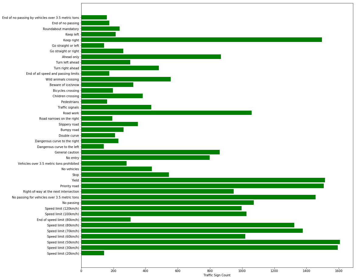
The training set consist of several sets of traffic signs and understanding how they are distributed was the initial step. The following is a bar chart showing the training data set. It is very evident that some signs have a larger dataset when compared to others.
Design and Test a Model Architecture
1. Pre processing techniques
The following are three pre processing techniques used in the model.
- Image Augmentation
- Colour Space
- Normalisation
Image Augmentation
In real life scenario a camera mounted on different vehicles such as passenger car or truck has different perspective of the traffic sign images. Three image augmentation methods were tested
- Image Translation - Needed as the traffic sign could be partially blocked in the field of view of the camera. The effect of translation is illustrated by an example image before and after the pre processing.

- Image Rotation - Mild rotation is needed as there are situations the traffic sign is seen from an uneven road gradient or traffic sign damaged by weather conditions. The effect of Rotation is illustrated by an example image before and after the pre processing.
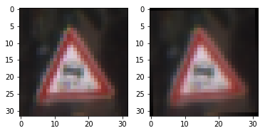
- Image Enhancement - The camera records the images in combination with different lighting conditions, exposure etc., The image need not be always sharp. A gaussian blur filter is a very effective method to reduce noise and smoothen the given image. The following is an example of the enhancement on a traffic sign.
Colour Space
- Grayscale - Grayscale is an effective means to improve the model performance in training for a feature but also faster training as the matrix is simplified. The training set was converted to grayscale.
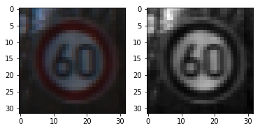
- HSV and YUV - Other colour space attempted to improve the features to standout for the model to be more robust in training.
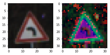
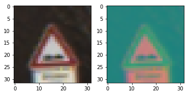
The different colour space did not yield promising results as expected. This may be possibly that the small features are better represented in RGB space than gray scale for the model.
Normalisation
The final step in the pre processing methods is to identify normalisation methods. Two different normalisation methods was experimented.
-
Feature Score - This normalisation is one of the most common and works better when the data is normally distributed.
-
Min Max Scaler or Feature Scaling - Feature scaling is used to bring all values into a range of [0,1]. It is also called unity based normalisation.
The feature score method performed better than min max scaler and hence it was used in the final preprocessing.
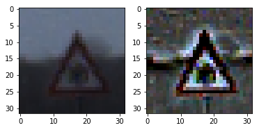
In order to build a robust model, the training data set should also be robust. The training set was augmented and concatenated to make twice the size of training data, which have images that are blurry, unsharp but also an equivalent preprocessed alias.
The following is an example of an original image and an augmented image:
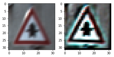
The difference between the original data set and the augmented data set is the following …
2. Model Architecture
I used the existing architecture of LeNet 5. A modification was made in the number of input as 32x32x3 and the output classes as 43.
My final model consisted of the following layers:
| Layer | Shape | Description |
|---|---|---|
| Input | 32x32x3 | RGB Image |
| Convolution | 28x28x6 | 1x1 Stride, Valid Padding |
| Activation | 28x28x6 | ReLU |
| Max Pooling | 14x14x6 | 2x2 Stride, Valid Padding |
| Convolution | 10x10x16 | 1x1 Stride, Valid Padding |
| Activation | 10x10x16 | ReLU |
| Max Pooling | 5x5x16 | 2x2 Stride, Valid Padding |
| Flatten | 400 | |
| Fully Connected | 120 | |
| Activation | 120 | ReLU |
| Fully Connected | 84 | |
| Activation | 84 | ReLU |
| Fully Connected | 43 | |
| Softmax | 43 | ReLU |
3. Training Model
The pipeline was implemented as Python class that enabled to instantiate different objects and experiment with hyper parameters.
Initially the model was trained with no change in the hyper parameters from the LeNet lab exercise. A baseline score was established on the model performance
A trial and error method to approach on a final value of the hyper parameters as below.
- Epoch 100
- Batch size 128
- mu 0
- Sigma 0.1
- Dropout 0.5 (50%)
- Adam Optimiser
- Learning Rate 0.001
4. Achieving > 0.93% accuracy
After the final training run the model was able to reach the desired accuracy level
My final model results were:
- validation set accuracy of 0.949
- test set accuracy of 0.845
The model was originally built with LeNet 5 architecture, because it’s a proven architecture for character recognition. The traffic signs, when looked at very smaller feature level (filters with a stride of 1x1) share commonality with characters.
The initial problems faced by the model was overfitting for the given dataset.
The model was not able to reach a higher accuracy because the original dataset did not capture worst case possibilities. Image augmentation and normalisation and addition of dataset improved the model performance.
Modifying the learning rate of the optimiser and the addition of dropouts 50% made the model robust.
As a final run I adjusted the batch size and the number of epochs for the model to reach a better accuracy in the validation.
The model performed as expected, as the test set score and new test image from the web reached similar accuracy.
Test a Model on New Images
1. Test Images and ideas behind choosing them
The five traffic sign that I choose to test on the model are a speed limit, general caution, priority road, road work and stop signs. The following is the test images after rescaling and augmentation.

The speed sign was chooses for two reason. This is the sign that model can be frequently subjected and with various number sign with similar characteristics, the model can predict it incorrectly. For example the image with speed sign 50 could appear as 80 with right level of noise and angle. The image also had a watermark, which could potentially reduce the softmax probability
The seconds image was “General Caution”. This was one of the interesting choices because there many similar looking signs in the dataset. For example Road narrows left, Road Narrows Right or Traffic Signal could appear as General caution sign to a model. The exclamation feature in the center of the triangle has similarity to many other warning signs.
The priority traffic sign was one the unique in the data set. A priority sign and end of priority sign are the only two that has a Rhombus shape. double border and two colour. This sign was probably the most unique for the model to predict. This sign also had part of the roof of the building that would have contaminated the prediction with other signs.
The road work was the favourite choice road sign because in reality there are usually multiple sign combined in a construction zone. In the test image there is barricade that could be seen as level crossing sign. The road work image as share its similarity of a person in the center with pedestrians and children’s crossing sign.
The fifth image is a stop sign. This also has unique octagon shape, with stop letters as characters. In general the LeNet 5 architecture performs very well for letter. Hence this is an easy choice for the model to predict.
2. Model Predictions
The following are the results of the prediction from the model.
| Image | Prediction |
|---|---|
| Speed Limit 50 Kmph | Speed Limit 50 Kmph |
| General Caution | Traffic Signal |
| Priority Road | Priority Road |
| Road Work | Road Work |
| Stop Sign | Stop Sign |
The model was able to correctly guess 4 of the 5 traffic signs, which gives an accuracy of 80%. This compares favorably to the accuracy on the test set of 84.5%.
3. Softmax Probability and Understanding Predictions
The code for making predictions on my final model is located in the last 4 cells 121, 22 and 41st result cell of the Ipython notebook.
The first image, the model is very sure that this is a speed limit of 50 Kmph (probability of 0.99), and the image does contain a 50 Kmph sign. The top five soft max probabilities are below. There was significantly low chance this image could be 80 kmph speed sign. The augmentation of the image cleared up the watermark.
| Prediction | Probability |
|---|---|
| Speed limit (50km/h) | 0.99996674061 |
| Speed limit (80km/h) | 0.00003324157 |
| Speed limit (100km/h) | 0.00000000000 |
| Speed limit (30km/h) | 0.00000000000 |
| Speed limit (60km/h) | 0.00000000000 |

The second image was general caution but the model incorrectly identified as traffic signal with very high confidence. This could potential be due to the close resemblance of General caution and traffic signal signs. More learning situations improvement in image augmentation can help address the situation.
| Prediction | Probability |
|---|---|
| Traffic signals | 0.99986636639 |
| General caution | 0.00013365022 |
| Pedestrians | 0.00000000000 |
| Speed limit (20km/h) | 0.00000000000 |
| Speed limit (30km/h) | 0.00000000000 |

The model was 100 % confident that the third image was Priority road and it correctly predicted this traffic sign. This might be due to the very unique shape and characteristics of this traffic sign.
| Prediction | Probability |
|---|---|
| Priority road | 1.0000000000 |
| Speed limit (20km/h) | 0.0000000000 |
| Speed limit (30km/h) | 0.0000000000 |
| Speed limit (50km/h) | 0.0000000000 |
| Speed limit (60km/h) | 0.0000000000 |

The fourth image was correctly predicted as with probability of 1.0 as road work. This was an interesting choice as this sign had chances to be predicted wrong due to the background of the image and other similar signs.
| Prediction | Probability |
|---|---|
| Road work | 1.000000000 |
| Right-of-way at the next intersection | 0.000000000 |
| Turn right ahead | 0.000000000 |
| Children crossing | 0.000000000 |
| Road narrows on the right | 0.000000000 |

The fifth image was the stop sign and model predicted with very high certainty that it was a stop sign.
| Prediction | Probability |
|---|---|
| Stop | 0.99997258186 |
| No entry | 0.00002637984 |
| Speed limit (120km/h) | 0.00000104451 |
| No passing | 0.00000000176 |
| No passing for vehicles over 3.5 metric tons | 0.00000000002 |
