Vehicle Detection
This project consists of constructing a pipeline using using OpenCV and Sklearn libraries to identify vehicles in a video stream.
The goals / steps of this project are the following:
- Explore and understand the given dataset of car and not a car image dataset.
- Perform a Histogram of Oriented Gradients (HOG) feature extraction on a labeled training set of images.
- Train a classifier using the dataset to determine if a given image is car or not a car.
- Define a pipeline to process a given image to identify if it has a car.
- Estimate a bounding box for the vehicles detected.
- Reduce the false positives in the identification.
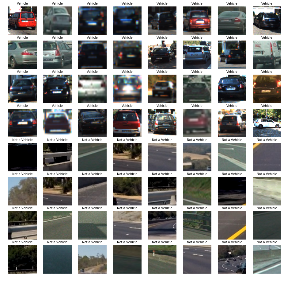
Explore the dataset
The first step is to explore and understand the given dataset, size of the images, visualize a few samples of car and not a car images. The following is a plot to show the samples of the images.
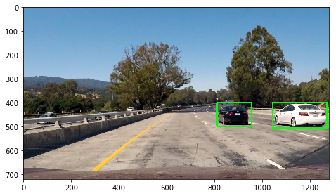
A function to draw rectangle is defined in the function draw_rectangle in cell 3. The following is an example of box around a given region.
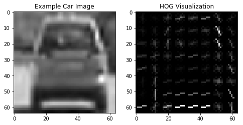
Histogram of Oriented Gradients (HOG)
The HOG values of given image can act as a unique signature in identifying a specific appearance of a feature like car. The function to determine the hog feature of an image is defined by the function extract_hog_by_skimage and extract_hog_by_opencv in the notebook cells 12 and 16. The following is an example of HOG image of a car and not a car.
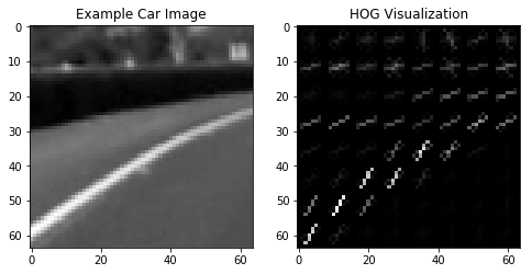
A different combination of HOG parameter were evaluated as shown below in the table.
| Configuration | color space | orientation | pix per cell | cell per block | channel | Extract_Time |
|---|---|---|---|---|---|---|
| 0 | YUV | 9 | 8 | 2 | ALL | 84.154645 |
| 1 | YUV | 9 | 8 | 2 | 0 | 26.747634 |
| 2 | YUV | 9 | 8 | 2 | 1 | 27.399855 |
| 3 | YUV | 9 | 8 | 2 | 2 | 27.281057 |
| 4 | YUV | 9 | 16 | 2 | ALL | 49.047909 |
| 5 | YUV | 9 | 16 | 2 | 0 | 16.573284 |
| 6 | YUV | 9 | 16 | 2 | 1 | 16.791569 |
| 7 | YUV | 9 | 16 | 2 | 2 | 17.329109 |
After finalizing on the parameter, HOG extraction using open CV hog function was also evaluated. The extraction time of the openCV function was significantly faster for the same requirements.
| Configurations | color space | orientation | pix per cell | cell per block | channel | Extract_Time |
|---|---|---|---|---|---|---|
| 0 | YUV | 9 | 8 | 2 | ALL | 5.052052 |
| 1 | YUV | 9 | 16 | 2 | ALL | 6.059657 |
In the final pipeline openCV HOG method was used to extract the features with “ALL” channels as more information could be extracted our of it.
Training a Classifier
The given feature set ylabels are classified in to two types cars and non-cars. The ylabels are given a value of 1 for cars and 0 for non-cars. The sklearn train_test_split functions is used to spilt the data and into training and test sets. In order to train the dataset on a classifier feature normalization was performed using the sklearn.preprocessing.StandardScaler. The scaler normalized the data to zero mean and unit variance. This helps the optimizer to converge correctly. Below are the images for scaled feature set.

2 different classifiers where trained to see the performance of the predictions.
- LinearSVC
- MultiLayer Perceptron
The function definitions can be found in the notebook cells 26 to 33. The performance of MLP was significantly better when compared to SVM. The confusion matrix for the MLP can be found below.
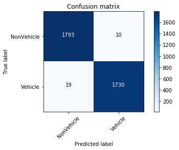
The classifier that was fit with training data and scaler functions are pickled as files and can be loaded for the pipeline search. In the final pipeline the MLP classifier was used based on the accuracy and the speed for predicting one test image sample was not much different between the LinearSVC or MLP.
Sliding Window Search
The sliding window search is implement in the function slide_window. The original function was adapted to cover the region with different scaling of the windows. Several window sizes and overlap percentages was explored. The functions are in notebook cells 33 to 39. An example of the sliding window applied to an image below.

False Positive elimination
The original detected windows are used create masked heat-map to identify the vehicle position. scipy.ndimage.measurements.label() was used to isolate the individual blobs. A threshold was applied to eliminate false positive identifications. A bounding box was constructed around each blob. Below is an image of false positive heat map and eliminated equivalent of the same

The amount of false positive detections are also reduced by selecting a specific softmax probability of the MLP classifier to a conservative value to be considered as a vehicle. Below of three examples of vehicle detected with its bounding boxes.


Video Implementation
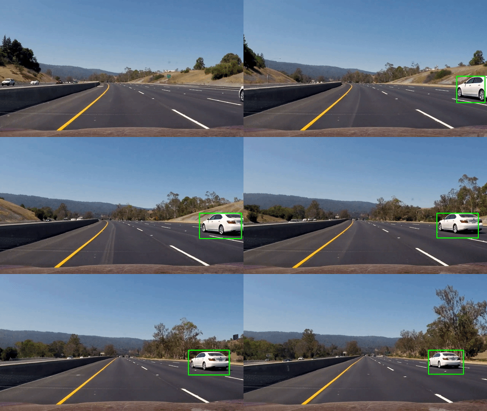
The link to the project video output Link to Video Result
The final implementation of the entire pipeline is implemented as python package with several class definition in the folder vehicleDetector. The package has Detector class and it can be generalized to be used with more updated classifier used in the future. This module also contains a box class which has double ended queue that holds the old frame detected boxes and it is used in the smoothing operation of the bound boxes for detected vehicle.
Discussion
The following are the situations that the pipeline might not be robust,
- The dataset contains only cars and non cars, in reality the road is shared by several different vehicles. The pipeline will fail to detect if a new vehicle is present in the lane.
- When a large dataset is used to train the classifier much better detection can be achieved, but it will be a balance of detection speed and accuracy. may be building a better classifier based on conv net using tensor flow might help to improve performance without compromise on speed.
- In adverse weather conditions the images will appear blurry and can change the Hog value of the features. A much larger dataset with varying weather and lighting conditions can be used as input or image augmentation can be used as input to improve the detection.
- There are edge case situation such as identifying vehicle in deep curves, vehicle being towed facing opposite direction etc. Possible performing a sensor fusion with radar data might help.
- While considering a real time implementation a balance between accuracy and speed has to be achieved.